Understanding the continuous phenological development at a daily time step with a Bayesian hierarchical space-time model: impacts of climate change and extreme weathers
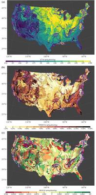
 Title: The sensitivity of speed of spring phenology to the changing rates of (a) daily maximum temperature anomaly (b) daily minimum temperature anomaly across the 914 ecoregions in the CONUS. The breaks of the color legend were selected to ensure that there were similar number of ecoregions within each color categories. Purple polygon boundary pointed out that the covariate is not significant in that eco-region (the 95% Bayesian posterior credible interval contains zero).
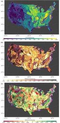
Abstract
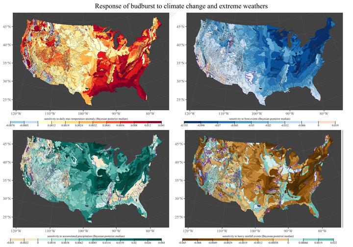
The impacts of climate change and extreme weather events (e.g. frost-, heat-, drought-, and heavy rainfall events) on the continuous phenological development over the entire seasonal cycle remained poorly understood. Previous studies mainly focused on modeling key phenological transition dates (e.g. discrete timing of spring bud-break and fall senescence) based on aggregated climate variables (e.g. mean temperature, growing-degree days). We developed and evaluated a Bayesian Hierarchical Space-Time model for Land Surface Phenology (BHST-LSP) to synthesize remotely sensed vegetation greenness with climate covariates at a daily temporal scale from 1981 to 2014 across the entire conterminous United States. The BHST-LSP model incorporated both temporal and spatial information and exhibited high predictive power in simulating daily phenological development with an overall out-of-sample R2 of 0.80 ± 0.17 and 0.72 ± 0.20 for spring and fall phenology, respectively. The overall out-of-sample normalized root mean square errors were 9.3% ± 6.1% and 9.9% ± 5.2% between the observed and predicted vegetation greenness for spring and fall phenology, respectively. We found that a fast increase of temperature can accelerate the speed of spring green-up while a slow decrease of temperature can lead to a decelerated fall brown-down. Increasing accumulated precipitation can benefit daily phenological development over an entire growing season, while extreme rainfall events can have the opposite effects. More frequent frost events could slow spring leaf expansion and accelerate fall leaf senescence. Impacts of extreme heat events were complex and depended on water availability. Cropland in the Midwest as well as evergreen needleleaf forest along the coastal regions showed relatively strong resistance to drought events compared to other land cover types. The BHST-LSP model can be used to forecast vegetation phenology given future climate projection, thus providing valuable information for adopting climate change adaptation and mitigation measures.
Research Highlights
- A Bayesian model was developed to simulate continuous phenological development.
- Rate of daily temperature changes impact speed of both spring and fall phenology.
- Increased precipitation benefit phenological development over an entire season.
- Frost events slow spring leaf expansion and accelerate fall leaf senescence.
- Cropland and evergreen forest show resistance to drought events.
Key innovations
The timing of spring and autumn transitions based on greenness measured by remote sensing are two metrics to characterize the phenology. There are many more important phenology characteristics that cannot be depicted by these two metrics. Additionally, the contributions from climate factors could vary continuously across the green-up or brown-down period (Clark et al., 2014a; Clark et al., 2014b; Friedl et al., 2014; Fu et al., 2015b; Seyednasrollah et al., 2018), degree-day models often overlooked such effects and summarized the entire times series of climate conditions to a single metric. The proposed Bayesian hierarchical space-time land surface phenology model simulated LSP as a continuous development process (Clark et al., 2014a) driven by daily climate covariates. In doing so, it was capable of attributing the contribution from a variety of environmental drivers, as well as their uncertainties, in influencing the rate of LSP, such as frost, drought and heat waves. Moreover, the BHST-LSP model incorporated a novel spatial component that enables us to “borrow strength” from neighboring pixels (Hammond et al., 2018) as well as to solve the “big-n” issue in remotely sensed big data, thus maximizing the capability of satellite observations in monitoring vegetation dynamics at a regional-to-continental scale. Additionally, we included the observation error in the first layer of the BHST-LSP model, making it robust to random noise in the model. It should also be noted that we can derive the timing of phenological transition dates from the predicted latent daily states from the BSHT-LSP model, given a user-defined threshold (e.g. 20% of the seasonal amplitude).
Accuracy is very high in the following figures